Having read this article, you will be able to implement blocked matrix multiplication and also to understand the number of memory accesses encountered in blocked matrix multiplication. In my next article, I will explain how these ideas can be extended to SIMD (Single Instruction Multiple Data) vector instructions.
Why is Matrix Multiplication Important?
Matrix multiplication is used in many scientific applications and recently it has been used as a replacement for convolutions in Deep Neural Networks (DNNs) using the im2col operation.
Matrix Storage
There are two ways of storing a dense matrix in memory. A dense matrix is where all / significant percentage (>40%) of the elements are non zeros. Sparse matrices can be stored in space efficient manners exploiting characteristics of zero. But, in this article, we will stick with dense matrices.
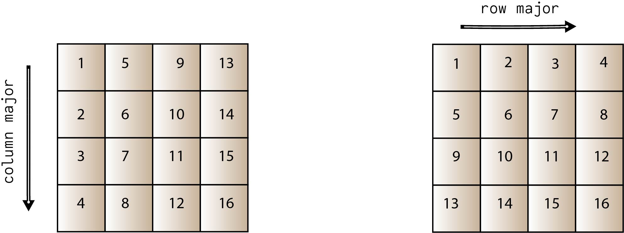
In the column major order, values are stored sequentially following the column order. Likewise, in row major, values are stored sequentially following row order. Order is important because of how these values are stored in memory. For efficient access, it is vital that the algorithms are aware of the underlying storage pattern.
Simple Memory Optimization Model
We will assume two levels of memory for simplicity: fast and slow. You can think as these to be the RAM and one level of cache. Initially data is stored in slow memory. We will define the following.
m = number of memory elements moved between slow and fast memory tm= time per slow memory operation f = number of arithmetic operations tf = time per arithmetic operation q = f/m (average number of flops per slow memory access)q factor is also known as the “computational intensity” and it’s vital to algorithm efficiency because per slow memory access we are intend to do more arithmetic operations.
Minimum possible computation time = tf * f (assuming the requested memory is already in fast memory) Actual computation time = computational cost + data fetch cost = f * tf + m * tm = f * tf ( 1 + (m * tm) / (f * tf)) = f * tf ( 1 + tm/tf * 1/q) —– equation (1)tm/tf is known as machine balance and is important to ensure machine efficiency. Therefore, we observe that memory efficiency depend on both machine balance and computational intensity. With higher q values, we can approach the theoretically possible minimum execution time.
To achieve half of the peak speed,
peak computation time >= data fetch cost
f * tf >= data fetch cost
f * tf >= f * tf * tm/tf * 1/q —– from equation (1)
q >= tm/tf
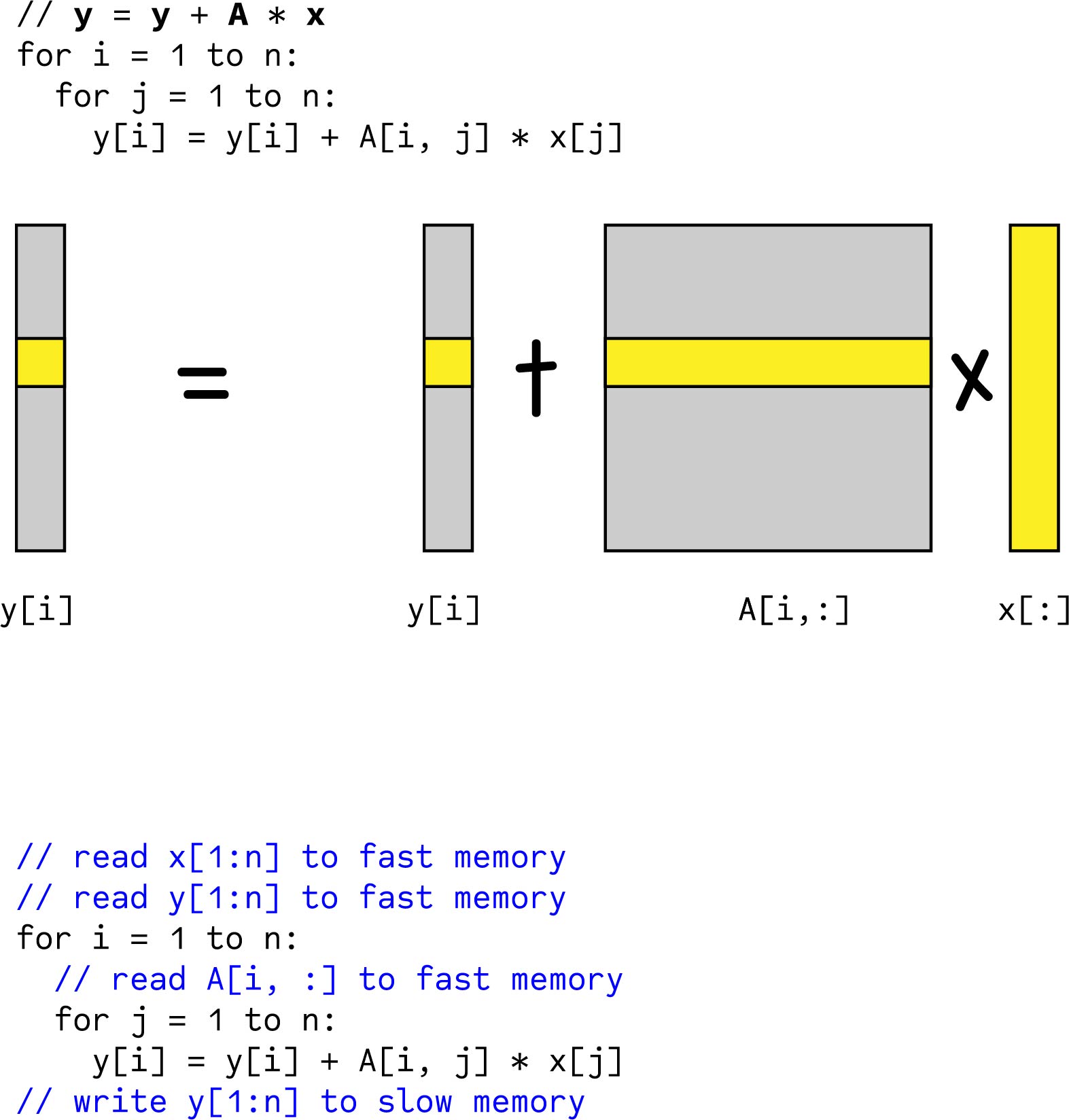
Matrix Vector Multiplication
Let’s first look at matrix vector multiplication. Each multiplication requires a prefetch of y vector and x vector to fast memory. Depending on the inner loop i, A matrix lines are loaded to fast memory.
In equation (2), slow memory accesses dominate the flops that can be achieved because tf amounts to a 1-2 clock cycles.
tm could amount to ~100 clock cycles.
Simplified Assumptions
In building this mental model, we made a few assumptions. Namely,
1. Assuming fast memory was large enough to hold three vectors.
Given the cache sizes of modern systems and that we are not dealing with infinitely large arrays, this claim holds to be true.
2. Cost of fast memory is virtually zero and this might be true for registers, but L1 and L2 cache requires 1~2 cycles.
3. Memory latency is constant.
Memory latency could vary based on the level of cache conflicts, processes in memory.
4. Ignoring between parallelism between memory and arithmetic operations. For example, DMA (Direct Memory Access) can relieve the CPU of data move tasks.
Matrix – Matrix Multiplication (Without Blocking)
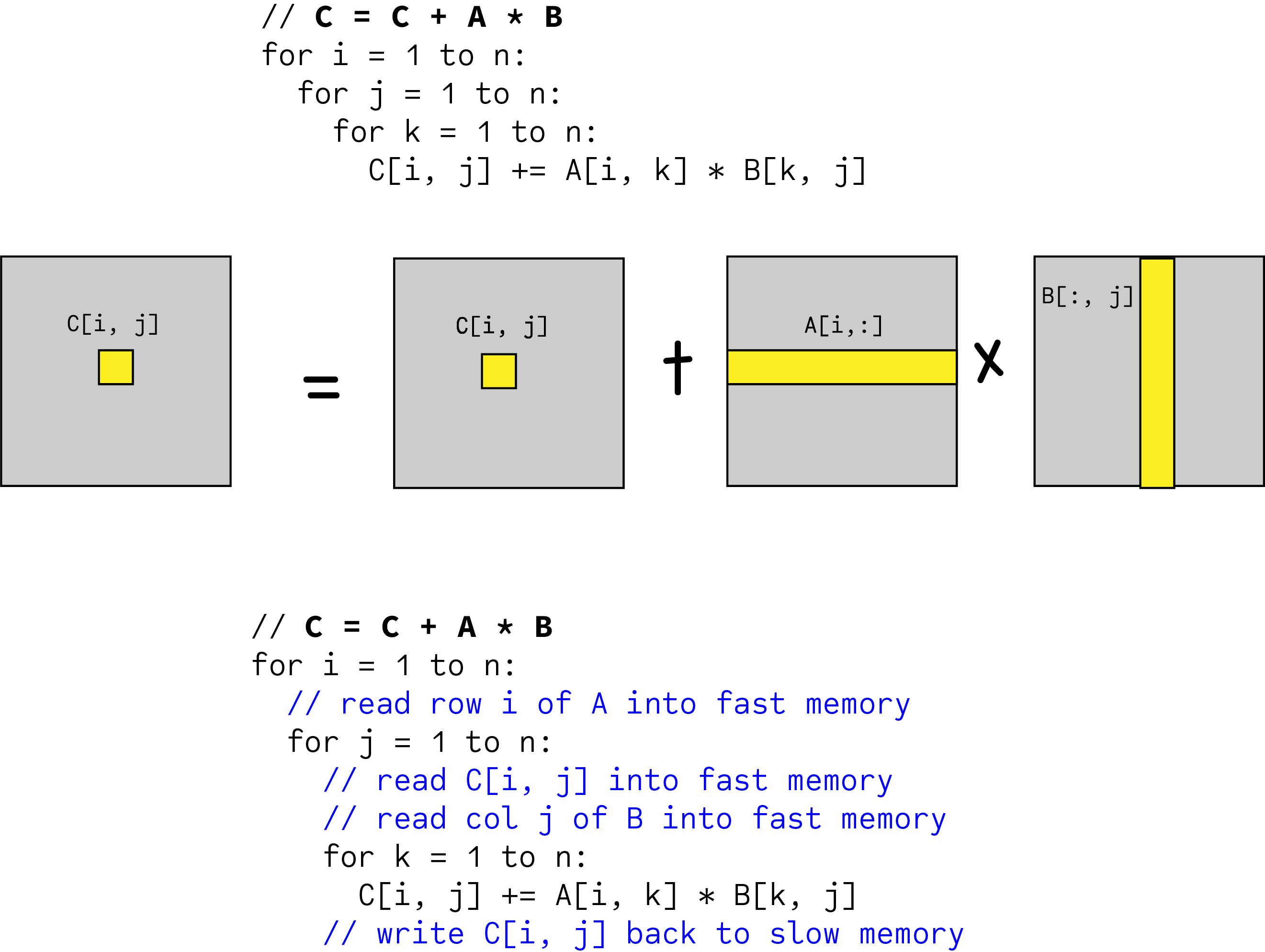
Number of slow memory references,
m = n3 + // read each col of B n times (one column has n elements and across i and j it accesses n2 times)
n2 + // read each row of A n times (one row has n elements and across i, it accesses n times)
2n2 // to read and write each element of C once
q = f / m = 2n3 / (n3 + 3n2) ~= 2 (so not significantly different from matrix – vector multiplication)
Blocked Matrix Multiplication
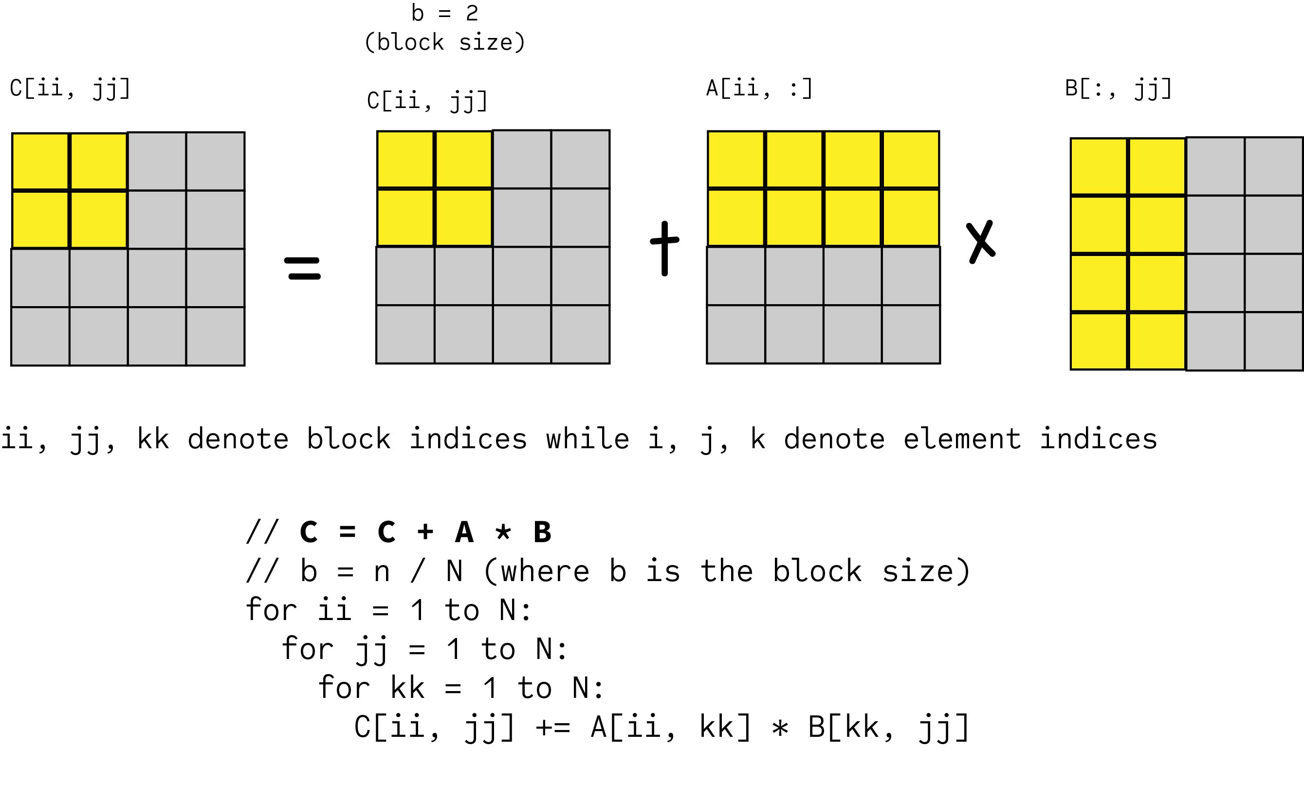
When implementing the above, we can expand the inner most block matrix multiplication (A[ii, kk] * B[kk, jj]) and write it in terms of element multiplications.
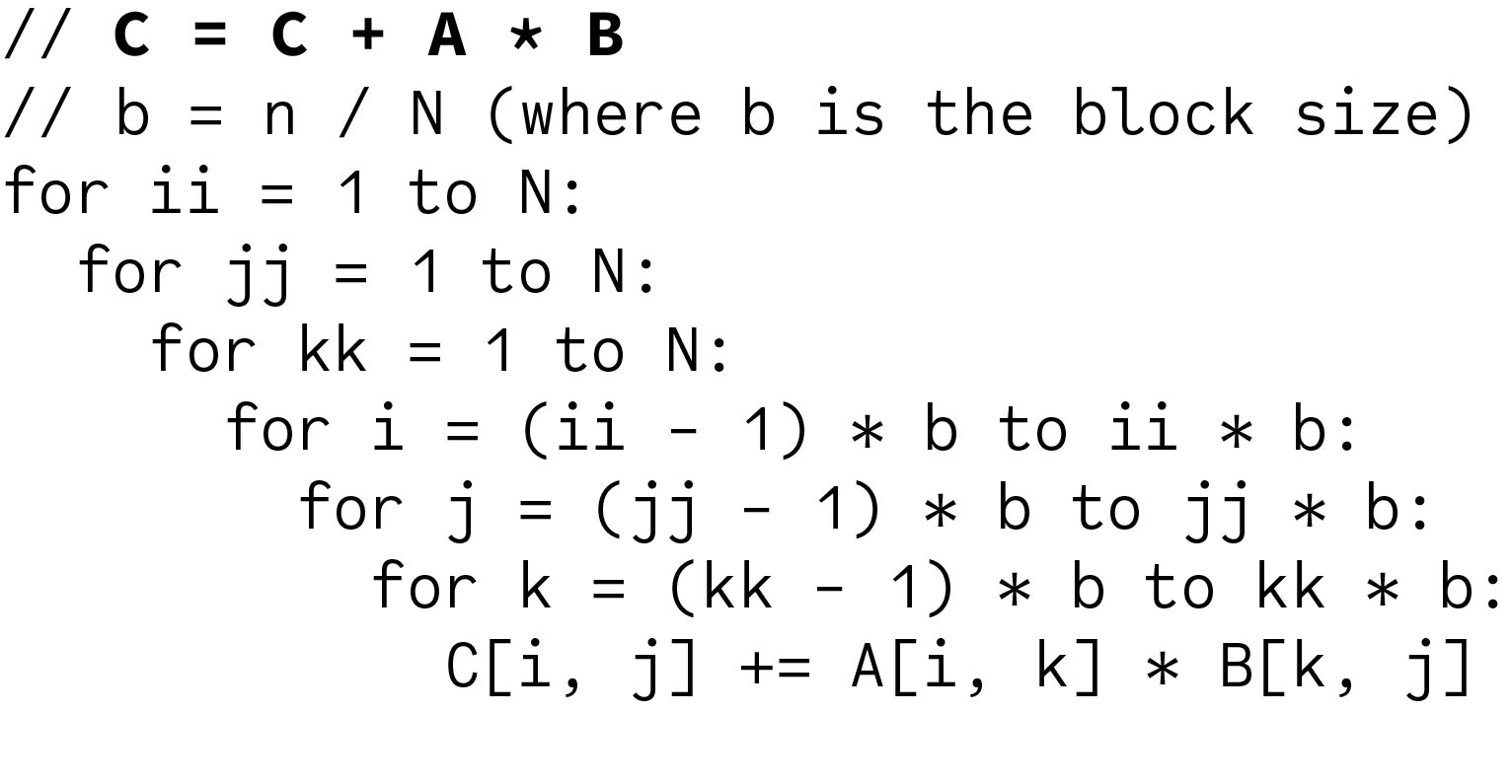
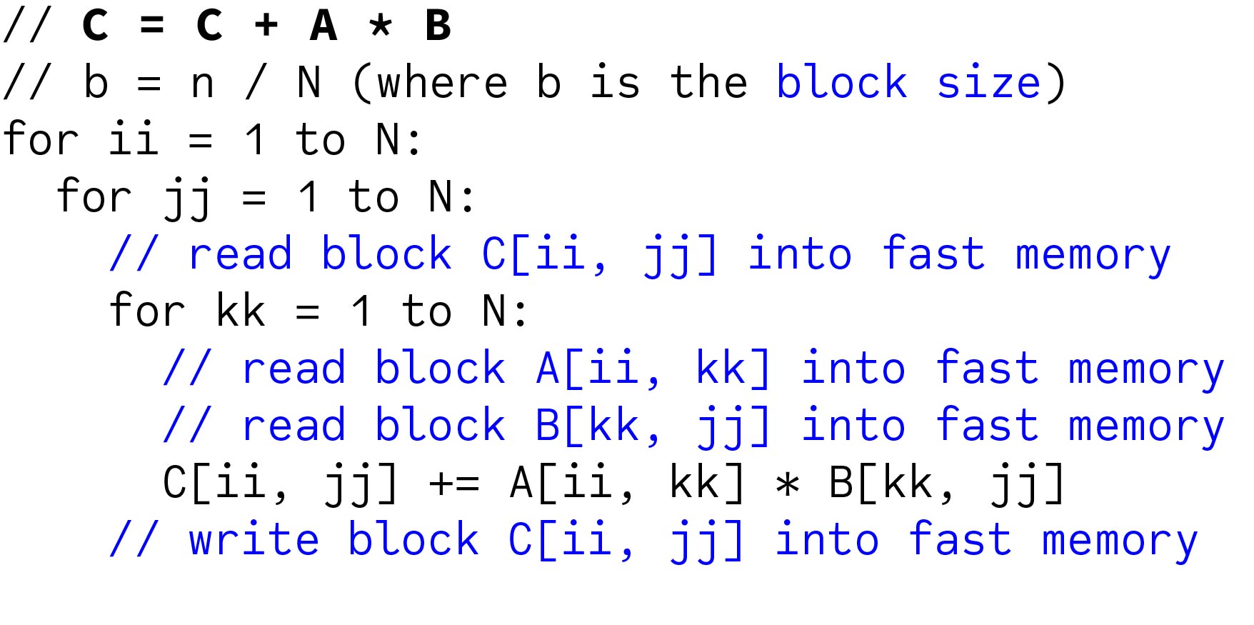
Next, we will analyze the memory accesses as we did before. The major difference from an unblocked matrix multiplication is that we can no longer hold a whole row of A in fast memory because of blocking. For each iteration of kk, we will need to load A[ii, kk] into fast memory. However, blocking increases computational density.
Simplified Analysis
memory transfers between fast and slow memory, m = N * n2 + // read each block of B N3 times (=N3 * (n / N)2 = num of times * elems per block) N * n2 + // read each block of A N3 times (=N3 * (n / N)2 = num of times * elems per block) 2 * n2 + // read and write of each block of C (=2 * N2 * (n / N)2 = 2 * num of times * elems per block) m = (2N + 2) * n2Therefore, the computational intensity is,
q = f / m = 2n3 / ((2N + 2) * n2) ~= n / N = b for large n
This result is important as it shows that we can increase the computational intensity by choosing a large value for b and it can be faster than matrix vector multiply (q = 2).
However, we cannot make the matrix sizes arbitrarily large because all three blocks have to fit inside the memory. If fast memory has size Mfast 3b2 <= Mfast q ~= b <= (Mfast / 3)1/2To get half of the machine peak capacity, q >= tm/tf
Therefore, to run blocked matrix multiplication at half of the peak machine capacity,
3q2 ~= 3b2 <= Mfast
3(tm/tf)2 <= Mfast
Now you have a comprehensive understanding of blocked matrix multiplication. Don’t forget to leave a comment behind!
Thank you for your information! I have a quick question. What if b=n? Then I think the block matrix is the same as the entire matrix multiplication; however, why does the b=n case show better computational intensity(q=b=n) than the entire matrix multiplication? (q=2)
Very good question.
When b=n, effectively in blocked matrix multiplication, three outer most loops execute only once. Thus, the blocked matrix multiplication becomes a full matrix multiplication.
However, our simplified analysis has an implicit assumption that N > 1. Otherwise, reading block to C, A, B to fast memory does not have a meaning (because blocking is not available). Therefore, to derive the computational intensity for b=n, we have to refer to the previous explanation.
Hope this answers your question.